Causal inference · Price economics
Dunnhumby — price elasticity and promotion effectiveness
Elasticity for 147 categories, and a campaign evaluation whose first answer was wrong in a way the standard check endorsed.
- My role
- Independent analyst · Sole contributor
- Period
- 2026 · Approximately 2 weeks
- Engagement
- Self-directed case study; completed individually
Business objective: Quantify how demand responds to price by category, and establish whether coupon campaigns caused incremental spend or only described who was already spending.
My ownership: I completed this project independently from end to end: framed the question, prepared and validated the data, performed the analysis, built the reporting output, and wrote the recommendations and limitations.
Two questions a commercial team asks constantly, and the second one is far harder than it looks. How much does demand move when price moves? And did the promotion actually cause anything, or would those sales have happened anyway?
Most retail data cannot answer the second one, because there is no comparison group. This dataset records which households received each coupon campaign — and 916 of 2,500 received none at all.
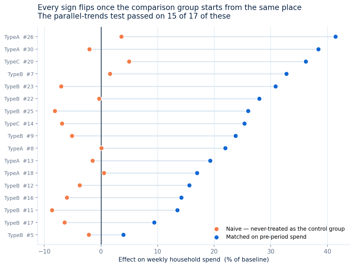
Own-price elasticity for 147 grocery categories, with display and mailer estimated in the same equation so each is purged of the others — 134 significant, median −0.71. The campaign evaluation’s first answer was that coupons reduced spend, and the parallel-trends test endorsed it on 15 of 17. The treated households had been spending 7× more before the campaign began. Matched on pre-period spend, every sign flips: 13 of 17 significantly positive, median +23.7%.
- Price, display and mailer in one equation.
log(units) = b·log(price) + g·display + d·mailer + product FE + week FE. All three together deliberately: a retailer discounts in the same week it features, so estimating price alone makes it absorb the display effect and the elasticity comes out too large. - Fixed effects, absorbed not dummied. Product effects absorb the difference between a 40-cent item and a 12-dollar one, so the estimate comes from a product being cheaper than its own normal price. Week effects absorb anything that moved every product at once. Both removed by alternating-projection demeaning, because a category can hold two thousand products across a hundred weeks.
- Difference-in-differences on the campaigns. Weekly household spend, treated against never-treated, eight weeks either side — with a parallel-trends test on the pre-period.
- Matching, after the first answer failed. Nearest-neighbour on pre-period weekly spend inside a 0.25 SD caliper, matching with replacement, effective sample size used in the standard error so reused controls do not inflate precision.
What the evidence says
What it found.
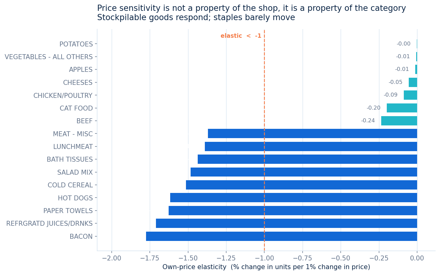
Stockpilable goods are elastic. Fresh meat is not
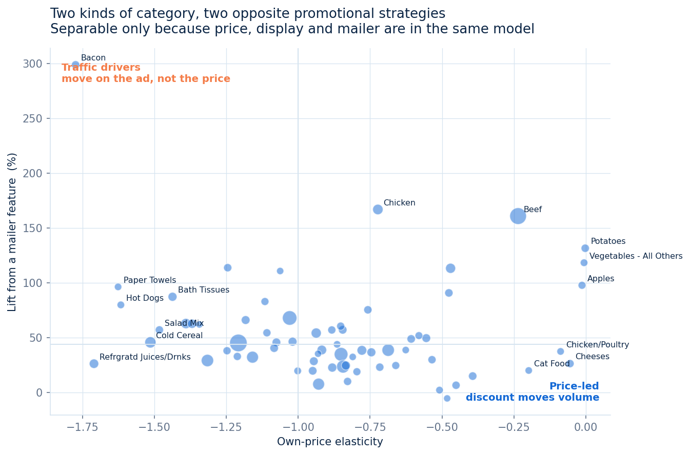
Bacon −1.77, refrigerated juice −1.71, cold cereal −1.51 — a shopper can buy bacon this week instead of next. Beef is −0.24 on price but moves +161% on the mailer: it is a traffic driver, bought because the trip happened. Those two facts imply opposite promotional strategies, and the model separates them only because display and mailer sit beside price.
The campaign answer was negative. Coupons do not do that
Twelve of 17 campaigns showed a negative effect, six significantly — up to −8.7% of baseline weekly spend. Not a surprising finding; a broken one.
The parallel-trends test passed on 15 of 17
The standard check gave the green light on exactly the campaigns producing an impossible answer. It is not a flawed test — parallel trends is a statement about slopes, and a comparison group averaging $10 a week has so little variance that its slope looks parallel to almost anything.
The diagnostic was looking at the levels
Treated households spent 7× more per week before the campaign started. The campaigns were targeted at the heaviest shoppers; the 916 who received nothing are a different population. What the naive estimate measured was heavy shoppers reverting toward their own mean.
Matched, every sign flips
Balance within $0.22 on bases of $44–76, against a 7× gap before. 17 of 17 positive, 13 significant, median +23.7% of baseline. Cost: 612 of 6,407 treated households dropped for having no comparable control — 9.6%, reported rather than absorbed.
What it looks like
The output, not a description of it.
- Elasticities are an upper bound on sensitivity. Retailers discount what they expect to sell, so demand the retailer anticipated gets attributed to the price cut. The promotion controls remove the main channel through which that happens, not all of it.
- The matched estimate is probably biased high, in the opposite direction to the naive one. Matching on a single noisy pre-period measure selects controls who happened to be having a good spell, and they revert down. The naive estimate is biased low; the truth sits between them.
- Fresh produce elasticities are measurement error, not behaviour. Potatoes −0.00, apples −0.01. Produce is sold by weight, so units and unit price are not comparable between baskets. Flagged, not dropped.
- Two of 147 categories return a positive sign and are flagged rather than reported. A positive own-price elasticity in a supermarket is a warning about the data, not a discovery about shoppers.
- A randomised holdout would settle the campaign question in one run, and that is the recommendation: hold out 10% of the targeted list and send them nothing.